Principal Component Analysis#
The intention of this notebook is to perform the PCA analysis on genotype data and generate plots.
Description#
Steps to generate a PCA include
removing related individuals
pruning variants in linkage disequilibrium (LD)
perform PCA analysis on genotype of unrelated individuals
excluding outlier samples in the PCA space for individuals of homogeneous self-reported ancestry. These outliers may suggest poor genotyping quality or distant relatedness.
Limitations#
Some of the PCs may capture LD structure rather than population structure (decrease in power to detect associations in these regions of high LD)
When projecting a new study dataset to the PCA space computed from a reference dataset: projected PCs are shrunk toward 0 in the new dataset
PC scores may capture outliers that are due to family structure, population structure or other reasons; it might be beneficial to detect and remove these individuals to maximize the population structure captured by PCA (in the case of removing a few outliers) or to restrict analyses to genetically homogeneous samples
Workflow#
Estimate relatedness of the individuals in the sample by PLINK 2 that implements the KING algorithm
Select specific SNPs and samples using PLINK and remove related individuals
SNPs thining by doing LD-pruning
The above steps are implemented in GWAS_QC.ipynb workflow.
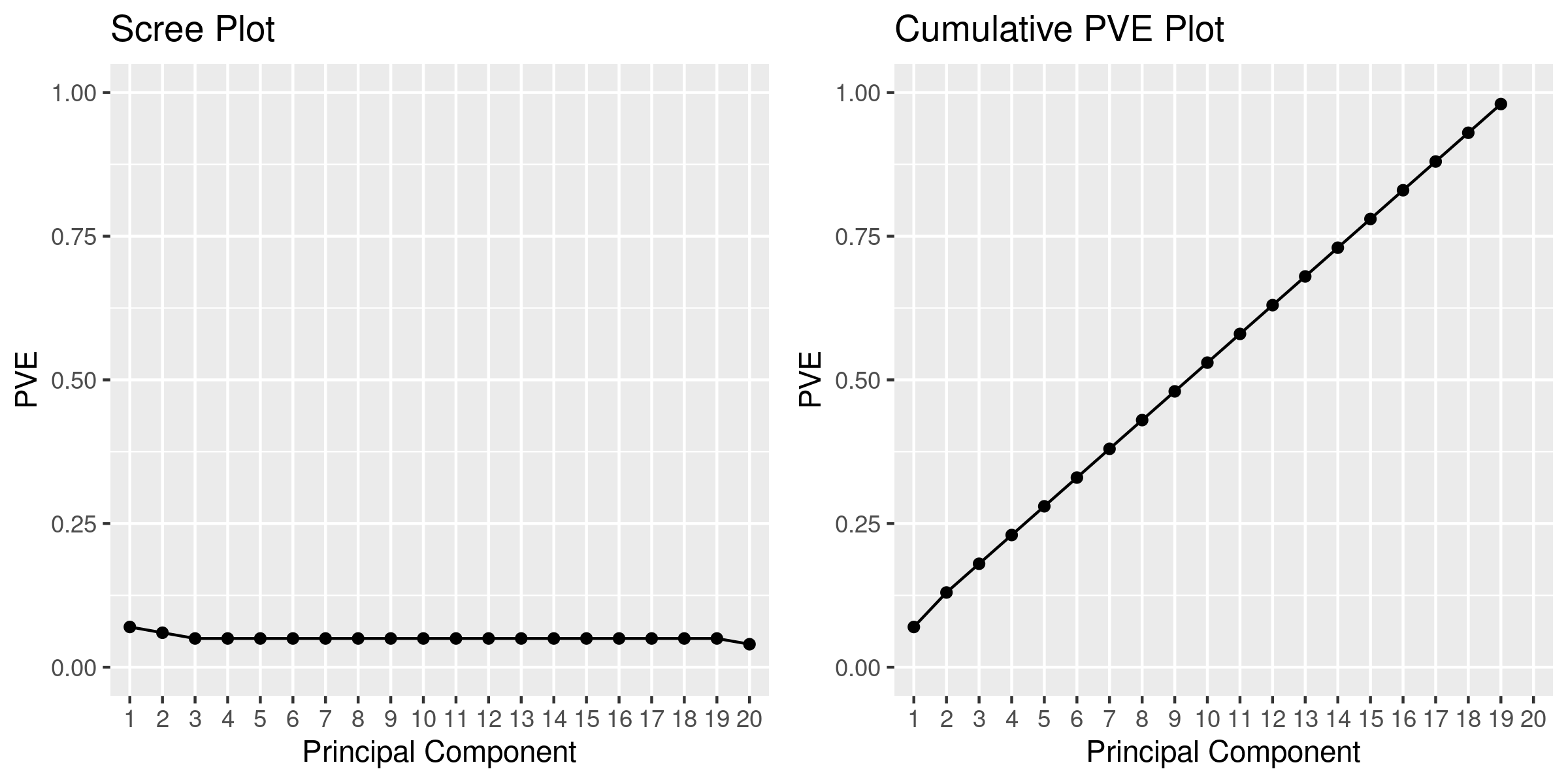
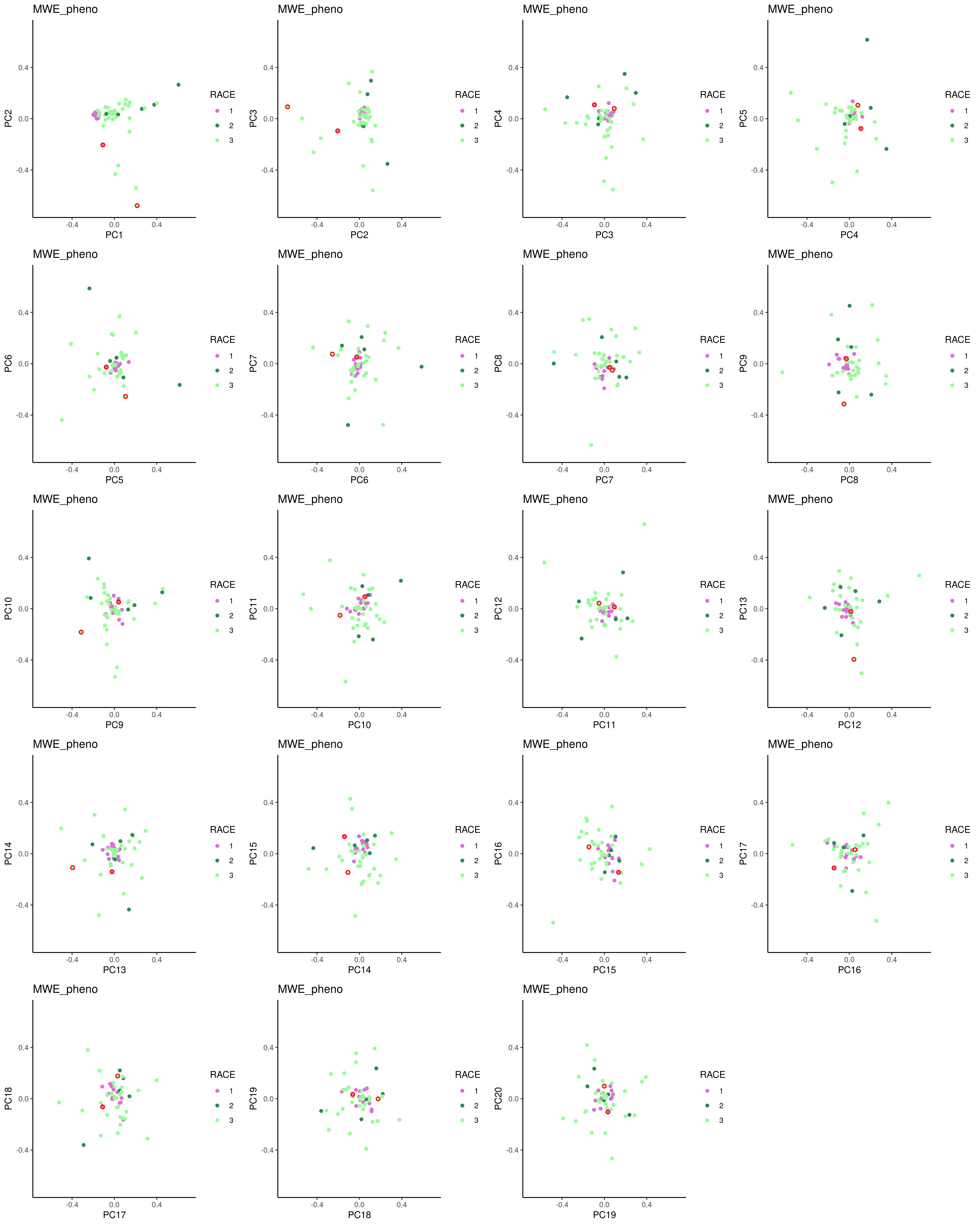
Run PCA using only unrelated individuals for all populations, and examine the resulting plot
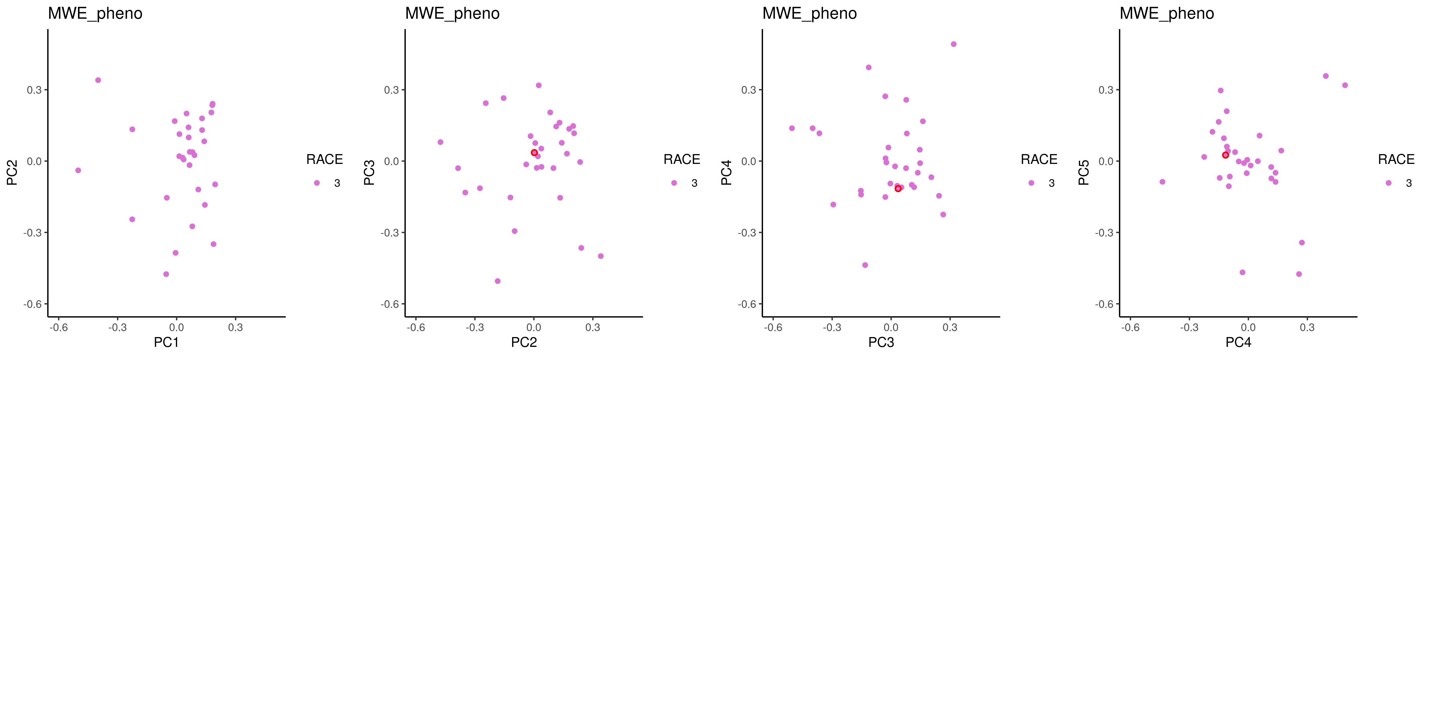
Project back related individuals, and generate a list of suggested samples to remove based on Mahalanobis distance test statistic per population. Default criteria is 0.997 percentile (two-sided) but we recommend checking the output plot before and after removal and rethink about it.
The analysis above can be performed with reference data eg 1000 Genomes integrated, to help diagnose population substructure in data.
If you have subpopulations in the data, then additional steps should be applied for:
Split data into different populations, each population data should have both related vs unrelated individual data-sets
For each population, perform QC
For each population, re-calculate per population PC’s for unrelated individuals
For each population, project related samples back to the PC space
Remove outliers based on list previously generated
Methods#
Here is a quick recap of PCA analysis for those not immediately familiar with the method. PCA is a mathematical method to reduce dimensionality of the data while retaining most of the variation in the dataset. This is accomplished by identifying directions or Principal Components (PC’s) that account for the maximum variation in the data.
One common approach to PCA is based on the singular-value decomposition of the the data matrix \(X\) (in our case the genotype matrix),
where \(U\) are the left eigenvectors, \(D\) is the diagonal matrix of singular values, and \(V\) are the right eigenvectors (also called loadings).
PCA can also be done using the eigen-decomposition of \(X X^T\):
where \(S=D^2\) is the diagonal matrix of eigenvalues. \(X\) is usually centred (mean-subtracted) or standardised (mean subtracted, then divided by standard deviation) before PCA.
For PCA of SNP genotypes (at least in diploid organisms), the common standardisation is
where \(X_{ij}\) is the genotype (minor allele dosage \(\{0, 1, 2\}\)) for the \(i\)th individual and the \(j\)th SNP, and \(p_j\) is the minor allele frequency (MAF) for the \(j\)th SNP. In addition, the eigenvalues are scaled by the number of SNPs \(m\) (equivalent to performing the eigen-decomposition of \(XX^T/m\)).
Input#
Genotype in PLINK format: common variants, LD pruned.
Phenotype files in text format and must contain a column ‘IID’ for individual ID. Optionally it can contain a column named ‘FID’ for family ID. In this case samples will be matched by both FID and IID. If you do not have a phenotype file you can input a PLINK fam file. The phenotype file can additionally contain population information and possibly disease or other labelling information, to label the PCA plots.
The inputs should be splitted into sets of related and unrelated individuals. Additionally you may want to prepare data per population. See “Minimal working example” section for more details.
Output#
PCA models (inside RDS file)
PCA scores (inside RDS file)
Mahalanobis distances and outliers to remove
Various plots
Minimal Working Example#
The data can be found on Synapse.
Note: parameters set for the MWE are meant to let the MWE work to show the workflow procedures. They may be unrealistic and should not be used in practice. The pipeline has reasonable default values for what we suggest to use in practice for most of the parameters.
Estimate kinship in the sample#
Identify and output closely related individuals prior to PCA analysis.
sos run GWAS_QC.ipynb king \
    --cwd output \
    --genoFile data/rename_chr22.bed \
    --kinship 0.13 \
    --name 20220110 \
    --container container/bioinfo.sif
Sample selection and QC the genotype data for PCA#
QC based on MAF, sample and variant missigness and Hardy-Weinberg Equilibrium. You can provide a list of samples to keep, or to remove. For example:
Only extract data for one population
Only extract data for related individuals
Only extract data for unrelated individuals In current context we would like to extract data for unrelated individuals and proceed with the rest of the QC steps.
LD pruning. Prune SNPs in linkage dissequilibrium to make sure the PCA actually captures population structure and not LD structure (which could reduce the power of detecting genetic associations in these LD-regions).
king will split data into unrelated and related individuals. We will QC on unrelated individuals but extract the same variants from related individuals. We therefore only run qc with a list of variants extracted, and other filtering parameters set to 0.
Finalize genotype QC by PCA for homogenous population#
Now pretend you analyze a homogenous population and you only did PCA to remove PC outliers. You have decided the outliers to remove and you would like to finalize the genotype QC.
First, remove these outliers and perform genotype data QC, similar to our initial QC but without LD pruning:
sos run GWAS_QC.ipynb qc_no_prune \
    --cwd output \
    --genoFile output/rename_chr22.20220110.unrelated.bed \
    --remove-samples output/pca/MWE_pheno.pca.projected.outliers \
    --name no_outlier \
    --container container/bioinfo.sif
Also remove outliers and keep the same variant as unrelated individuals, in related individuals:
sos run GWAS_QC.ipynb qc_no_prune \
    --cwd output \
    --genoFile output/rename_chr22.20220110.related.bed \
    --remove-samples output/pca/MWE_pheno.pca.projected.outliers \
    --keep-variants output/rename_chr22.20220110.unrelated.no_outlier.filtered.bim \
    --maf-filter 0 --geno-filter 0 --mind-filter 0.1 --hwe-filter 0 \
    --name no_outlier \
    --container container/bioinfo.sif
Finally, merge back related and unrelated individuals as finalized genotype in PLINK format,
sos run genotype_formatting.ipynb merge_plink \
    --genoFile output/rename_chr22.20220110.unrelated.no_outlier.filtered.bed \
               output/rename_chr22.20220110.related.no_outlier.filtered.extracted.bed \
    --cwd output/genotype_final \
    --name chr22_20220110_qced \
    --container container/bioinfo.sif
You can stop here if you’re analyzing a homogenous population.
Split data by population#
If your data contains multiple populations, then for each population, you can still use the GWAS_QC.ipynb and PCA.ipynb workflows, except that at this step you have to split data by population using manually created files to include or to remove samples.
pheno = read.table("data/MWE_pheno.txt", header = TRUE, stringsAsFactors=F)
for (i in 1:3){
 race = subset(pheno, RACE == i)
 race_id = cbind(race[,2],race[, 2])
 write.table(race_id, paste0("output/ID.", "race", i), quote = FALSE, sep = '\t', col.names = FALSE, row.names = FALSE)
}
For each population do their own QC to finalize#
Same as steps as the Finalize genotype QC by PCA for homogenous population step, taking into consideration of outliers detected. Please read the GWAS_QC.ipynb document to see available QC options and recommendations.
Command Interface#
sos run PCA.ipynb -h
[global]
# the output directory for generated files
parameter: cwd = path("output")
# A string to identify your analysis run
parameter: name = ""
# Name of the population column in the phenoFile
parameter: pop_col = ""
# Name of the populations (from the population column) you would like to plot and show on the PCA plot
parameter: pops = []
# Name of the color label column in the phenoFile; can be the same as population column. Can also be a separate column eg a "super population" column as a way to enable you to combine selected populations based on another column.
parameter: label_col = ""
# Number of Principal Components to output,must be consistant between flashpca run and project samples run (flashpca partial PCA method).
parameter: k = 20
# Number of Principal Components based on which outliers should be evaluated. Default is 5 but this should be based on examine the scree plot
parameter: maha_k = 5
# Homogeneity of populations. Set to --homogeneous when true and --no-homogeneous when false
parameter: homogeneous = False
# Software container option
parameter: container = ""
import re
parameter: entrypoint= ('micromamba run -a "" -n' + ' ' + re.sub(r'(_apptainer:latest|_docker:latest|\.sif)$', '', container.split('/')[-1])) if container else ""
# For cluster jobs, number commands to run per job
parameter: job_size = 1
# Wall clock time expected
parameter: walltime = "5h"
# Memory expected
parameter: mem = "16G"
# Number of threads
parameter: numThreads = 10
suffix = '_'.join(pops)
cwd = path(f"{cwd:a}")
if not pop_col:
    homogeneous = True
# PCA command with PLINK, as a sanity check
[pca_plink]
# PLINK binary file
parameter: genoFile = path
input: genoFile
output: f'{cwd}/{genoFile:bn}.pca.eigenvec'
task: trunk_workers = 1, trunk_size = job_size, walltime = walltime, mem = mem, cores = numThreads, tags = f'{step_name}_{_output[0]:bn}'
bash: container = container, expand = "${ }", stderr = f'{_output[0]:n}.stderr', stdout = f'{_output[0]:n}.stdout', entrypoint=entrypoint
    plink --bfile ${_input:n} --out ${_output:n} --pca ${k}
PCA analysis#
# Run PCA analysis using flashpca
[flashpca_1]
# Plink binary file
parameter: genoFile = path
# The phenotypic file
parameter: phenoFile = path(f'{genoFile}'.replace(".bed",".fam"))
# minimum population size to consider in the analysis
parameter: min_pop_size = 2
# How to standardize X before PCA
parameter: stand = "binom2"
## Input genoFile here is for unrelated samples
input: genoFile, phenoFile
output: f'{cwd}/{phenoFile:bn}{("."+name) if name else ""}.{(suffix+".") if suffix != "" else ""}pca.rds'
task: trunk_workers = 1, trunk_size = job_size, walltime = walltime, mem = mem, cores = numThreads, tags = f'{step_name}_{_output[0]:bn}'
R: container = container, expand = "${ }", stderr = f'{_output:n}.stderr', stdout = f'{_output:n}.stdout', entrypoint=entrypoint
    # Load required libraries
    library(flashpcaR)
    library(dplyr)
    pops = c(${paths(pops):r,})
    f <- flashpca(${_input[0]:nr}, ndim=${k}, stand="${stand}", do_loadings=TRUE, check_geno=TRUE)
    rownames(f$loadings) <- read.table('${_input[0]:n}.bim',stringsAsFactors =F)[,2]
    # Use the projection file to generate pca plot
    pca <- as.data.frame(f$projection)
    pca <- tibble::rownames_to_column(pca, "ID")
    colnames(pca) <- c("ID",paste0("PC", 1:${k}))

    # Read fam file with phenotypes
    if(stringr::str_detect(${_input[1]:r},".fam$")){
        pheno <- read.table(${_input[1]:r}, header=F,stringsAsFactors =F)
        colnames(pheno) = c("FID", "IID", "MID", "PID", "SEX", "STATUS")
    } else {
        pheno <- read.table(${_input[1]:r}, header=T,stringsAsFactors =F)
        if("IID" %in% colnames(pheno) == FALSE) stop("No IID column in the phenoFile. Please rename the header of the phenoFile")
        if("FID" %in% colnames(pheno) == FALSE) pheno$FID = pheno$IID
    }
    # Make the unique ID by merge FID and IID
    pheno$ID = paste(pheno$FID,pheno$IID,sep = ":")
    #check duplicated ID
    if(length(unique(pheno$ID))!=length(pheno$ID)) stop("There are duplicated names in IID column of phenoFile")

    if (length(pops)>0) pheno <- pheno %>%filter(${pop_col if pop_col else  "pop"} %in% pops | ${label_col if label_col else  "pop"} %in% pops)
    pca <-merge(pheno, pca,by ="ID", all=FALSE)
    #
    if (${"TRUE" if pop_col else "FALSE"}) {
        # remove populations have less than ${min_pop_size} samples
        pop<-names(table(pca$${pop_col if pop_col else "pop"}))
        pop_filter<-pop[table(pca$pop)<${min_pop_size}] # pop to be removed
        if (length(pop_filter)>0) {
            warning(for (i in pop_filter){cat(i,';')},'these ', length(pop_filter)," population will be removed due to having less than ${min_pop_size} samples in data.")
            # remove
            pca<-pca%>% filter(${f'!{pop_col}%in%pop_filter' if pop_col else pop_col})
        }
    } else {
      pca$pop <- 1
    }

    # Write the PC scores to a file
    write.table(pca,"${_output:n}.txt", sep="\t", quote=FALSE, row.names=FALSE, col.names=TRUE)
    dat = list(pca_model = f, pc_scores = pca, meta = "${_input[1]:bn} ${suffix}")
    # compute centroids before projecting back the samples
    # (calculate mean/median/cov per pop)
    if(${"FALSE" if homogeneous else "TRUE"}){
        pop_group <- split(dat$pc_scores[ ,c(paste0("PC", 1:${maha_k}))], list(Group = dat$pc_scores$${pop_col if pop_col else "pop"}))
        dat$pc_cov <- lapply(pop_group, function(x) cov(x))
        dat$pc_mean <- lapply(pop_group, function(x) sapply(x, mean))
        dat$pc_median <- lapply(pop_group, function(x) sapply(x, median))
    } else {
        dat$pc_cov <- cov(f$projection[,1:${maha_k}])
        dat$pc_mean <- apply(f$projection[,1:${maha_k}], 2, mean)
        dat$pc_median <- apply(f$projection[,1:${maha_k}], 2, median)
    }

    # save results
    saveRDS(dat, ${_output:r})

bash: expand= "$[ ]", stderr = f'{_output:n}.stderr', stdout = f'{_output:n}.stdout', container = container, entrypoint=entrypoint
        stdout=$[_output:n].stdout
        for i in $[_output] ; do
        echo "output_info: $i " >> $stdout;
        echo "This rds file is a list containing the pca for unrelated sample" >> $stdout;
        echo "output_size:" `ls -lh $i | cut -f 5  -d  " "`   >> $stdout;
        done
Plot PCA results#
# Plot PCA results.
# Can be used independently as "plot_pca" or combined with other workflow as eg "flashpca+plot_pca"
[plot_pca]
parameter: outlier_file = path()
parameter: plot_data = path
parameter: min_axis = ""
parameter: max_axis = ""
input: plot_data
output: f'{cwd}/{_input:bn}.pc.png',
        f'{cwd}/{_input:bn}.scree.png',
        f'{cwd}/{_input:bn}.scree.txt'
task: trunk_workers = 1, trunk_size = job_size, walltime = walltime, mem = mem, cores = 1, tags = f'{step_name}_{_output[0]:bn}'
R: container = container, volumes = [f"{outlier_file:ad}:{outlier_file:ad}"], expand = "${ }", stderr = f'{_output[0]:n}.stderr', stdout = f'{_output[0]:n}.stdout', entrypoint=entrypoint
    library(dplyr)
    library(ggplot2)
    library(gridExtra)
    library(matrixStats)
    pops = c(${paths(pops):r,})
    dat = readRDS(${_input:r})
    f = dat$pca_model
    pca_final<-dat$pc_scores

    if (length(pops)>1) pca_final <- pca_final %>% filter(${pop_col if pop_col else "pop"} %in% pops | ${label_col if label_col else  "pop"} %in% pops)
    pca_final <- pca_final %>% mutate(${label_col if label_col else "pop"}=as.character(${label_col if label_col else  "pop"}))
    k = ${k}
    # manually set colors for PCA plotting, to avoid similar colors in one plot:
    # generated by https://mokole.com/palette.html
    set.seed(999)
    colors_40 = sample(c("#a9a9a9", "#2f4f4f", "#556b2f", "#a0522d", "#7f0000", "#006400", "#808000", "#483d8b", "#3cb371", "#bdb76b", "#4682b4", "#9acd32",
                          "#20b2aa", "#00008b", "#32cd32", "#daa520", "#7f007f", "#b03060", "#ff0000", "#ff8c00", "#ffff00", "#0000cd", "#00ff00", "#9400d3",
                          "#00fa9a", "#00ffff", "#00bfff", "#f4a460", "#f08080", "#adff2f", "#ff6347", "#ff00ff", "#1e90ff", "#dda0dd", "#7b68ee", "#afeeee",
                          "#ee82ee", "#ff69b4", "#ffe4c4", "#ffc0cb"))
    colors_20 = sample(c("#2f4f4f", "#2e8b57", "#8b0000", "#808000", "#00008b", "#ff0000", "#ff8c00", "#00ff00", "#4169e1", "#00ffff", "#00bfff", "#0000ff",
                          "#da70d6", "#d8bfd8", "#ff00ff", "#eee8aa", "#ffff54", "#ff1493", "#ffa07a", "#98fb98"))

    # assign colors to each ethnicity:
    num_col=length(unique(pca_final$${label_col if label_col else "pop"}))
    if (num_col <= 20) {
       color_list <- colors_20[1:num_col]
    } else {
       color_list <- colors_40[1:num_col]
    }

    ###
    # Make the plots
    ###
    # Get the min and max values for x and y-axes
    if (${"TRUE" if len(min_axis) == 0 or len(max_axis) == 0 else "FALSE"}) {
        min_axis <- round(colMins(as.matrix(f$projection[sapply(f$projection, is.numeric)])),1)
        max_axis <- round(colMaxs(as.matrix(f$projection[sapply(f$projection, is.numeric)])),1)
    } else {
        min_axis <- as.double(${min_axis})
        max_axis <- as.double(${max_axis})
    }
    if (${"TRUE" if outlier_file.is_file() else "FALSE"}) {
        outliers <- read.table(${outlier_file:r}, col.names=c("FID", "IID"),stringsAsFactors =F)
        plot_pcs = function(pca_final, x, y, title="") {
            ggplot(pca_final, aes_string(x=x, y=y)) + geom_point(${f'aes(color={label_col})' if label_col else ""}) +
              # add circles for these ouliters:
              geom_point(data=filter(pca_final, IID %in% outliers$IID, FID %in% outliers$FID), shape = 21, size=1.5, color='red', stroke = 0.9) +
              # add outliers dots:
              geom_point(data=filter(pca_final, IID %in% outliers$IID, FID %in% outliers$FID), shape = 16, size=1${f',aes(color={label_col})' if label_col else ""} ) +
              labs(title=title,x=x, y=y) +
              scale_y_continuous(limits=c(min_axis, max_axis)) +
              scale_x_continuous(limits=c(min_axis, max_axis)) +
              scale_color_manual(values=color_list) +
              theme_classic()
        }} else {
        plot_pcs = function(pca_final, x, y, title="") {
          ggplot(pca_final, aes_string(x=x, y=y)) + geom_point(${f'aes(color={label_col})' if label_col else ""}) +
              labs(title=title,x=x, y=y) +
              scale_y_continuous(limits=c(min_axis, max_axis)) +
              scale_x_continuous(limits=c(min_axis, max_axis)) +
              scale_color_manual(values=color_list) +
              theme_classic()
        }}
    unit = 4
    n_col = min(4, k)
    n_row = ceiling(k / n_col)
    plots = lapply(1:(k-1), function(i) plot_pcs(pca_final, paste0("PC",i), paste0("PC",i+1), dat$meta))
    png('${_output[0]}', width = unit * n_col, height = unit * n_row, unit='in', res=300)
    do.call(gridExtra::grid.arrange, c(plots, list(ncol = n_col, nrow = n_row)))
    dev.off()
    # Create scree plot
    PVE <- f$values
    PVE <- round(PVE/sum(PVE), 2)
    PVEplot <- qplot(c(1:length(PVE)), PVE) + geom_line() + xlab("Principal Component") + ylab("PVE") + ggtitle("Scree Plot") + ylim(0, 1) +scale_x_discrete(limits=factor(1:length(PVE)))
    PVE_cum <- cumsum(PVE)/sum(PVE)
    cumPVEplot <- qplot(c(1:length(PVE)), cumsum(PVE)) + geom_line() + xlab("Principal Component") + ylab("PVE") + ggtitle("Cumulative PVE Plot") + ylim(0, 1) + scale_x_discrete(limits=factor(1:length(PVE)))
    png('${_output[1]}', width = 8, height = 4, unit='in', res=300)
    grid.arrange(PVEplot, cumPVEplot, nrow = 1)
    dev.off()
    ## Textual Output

    PVE_output = tibble(PCs = 1:length(PVE), PVE = PVE, PVE_cum = PVE_cum )
    PVE_output%>%readr::write_delim(${_output[2]:r},"\t")

bash: expand= "$[ ]", stderr = f'{_output[0]:n}.stderr', stdout = f'{_output[0]:n}.stdout' , container = container, entrypoint=entrypoint
        stdout=$[_output[0]:n].stdout
        for i in $[_output[2]] ; do
        echo "output_info $i " >> $stdout;
        echo "This is the PC score" >> $stdout;
        echo "output_size:" `ls -lh $i | cut -f 5  -d  " "`   >> $stdout;
        echo "output_rows:" `cat $i | wc -l  | cut -f 1 -d " "`   >> $stdout;
        echo "output_column:" `cat $i | head -1 | wc -w `   >> $stdout;
        echo "output_preview:"   >> $stdout;
        cat $i | head  | cut -f 1,2,3,4,5,6   >> $stdout ; done
Detect outliers#
# Calculate Mahalanobis distance per population and report outliers
[detect_outliers]
# Set the probability to remove outliers eg 0.95 or 0.997
parameter: prob = 0.997
# Mahalanobis distance p-value cutoff
parameter: pval = 0.05
# Robust Mahalanobis to outliers
parameter: robust = True
parameter: pca_result = path
input: pca_result
output: distance=f'{_input:n}.mahalanobis.rds',
        identified_outliers=f'{_input:n}.outliers',
        analysis_summary=f'{_input:n}.analysis_summary.md',
        qqplot_mahalanobis=f'{_input:n}.mahalanobis_qq.png',
        hist_mahalanobis=f'{_input:n}.mahalanobis_hist.png'
task: trunk_workers = 1, trunk_size = job_size, walltime = walltime, mem = mem, cores = 1, tags = f'{step_name}_{_output[0]:bn}'
bash: container = container, expand = "${ }", entrypoint=entrypoint
    echo '''---
    theme: base-theme
    style: |
      img {
        height: 80%;
        display: block;
        margin-left: auto;
        margin-right: auto;
      }
    ---
    ''' > ${_output[2]}

R: container = container, expand= "${ }", stderr = f'{_output[0]:n}.stderr', stdout = f'{_output[0]:n}.stdout', entrypoint=entrypoint
    # Load required libraries
    library(dplyr)
    library(ggplot2)
    library(gridExtra)

    # invert a known covariance matrix but allow them to be numerically singular matrix (still assuming full rank)
    robust_inv = function(s) {
        #tryCatch(solve(s), error=function(cond) solve(Matrix::nearPD(s)$mat))
        tryCatch(solve(s), error=function(cond) MASS::ginv(s))
    }

    # Calculate mahalanobis distance
    calc_mahalanobis_dist = function(x, m, s, name = '', prob=${prob}) {
        pc <- x %>%
          select("IID","FID", "${pop_col if pop_col else "pop"}", starts_with("PC"))
        mu_pc <- pc[,4:(4 + length(m) - 1)]
        pc$mahal = mahalanobis(mu_pc, m, robust_inv(s), inverted=TRUE)
        pc$p <- pchisq(pc$mahal, df=nrow(s), lower.tail=FALSE)
        manh_dis_sq_cutoff = quantile(pc$mahal, probs=prob)
        # Obtain outliers
        outliers = pc[(pc$mahal > manh_dis_sq_cutoff & pc$p < ${pval}),]
        d_summary = paste0(capture.output(summary(pc$mahal)), collapse = '\n')
        msg = paste('#', name, "result summary\n## Mahalanobis distance summary:\n```\n", d_summary, "\n```\n",
            paste("The cut-off for outlier removal is set to:", manh_dis_sq_cutoff, "and the number of individuals to remove is:", nrow(outliers),"\n"),
            paste("The new sample size after outlier removal is:",nrow(pc) - nrow(outliers),"\n"))
        #
        outliers <- outliers %>%
        select(FID,IID)
      list(pc=pc, manh_dis_sq_cutoff=manh_dis_sq_cutoff, msg=msg, outliers=outliers)
    }

    dat = readRDS(${_input:r})
    if (is.list(dat$pc_mean)) {
      pops = names(dat$pc_mean)
      pop_group = split(dat$pc_scores, f = dat$pc_scores$${pop_col if pop_col else "pop"})
      res = lapply(pops, function(p) calc_mahalanobis_dist(pop_group[[p]], dat$${"pc_mean" if not robust else "pc_median"}[[p]], dat$pc_cov[[p]], name = paste(dat$meta, p)))
      names(res) = pops
      res = list(
          msg = do.call(paste, c(lapply(pops, function(p) res[[p]]$msg), sep = "\n")),
          manh_dis_sq_cutoff = cbind(pops, sapply(pops, function(p) res[[p]]$manh_dis_sq_cutoff)),
          outliers = do.call(rbind, c(lapply(pops, function(p) res[[p]]$outliers))),
          pc = do.call(rbind, c(lapply(pops, function(p) res[[p]]$pc)))
          )
    } else {
      res = calc_mahalanobis_dist(dat$pc_scores, dat$${"pc_mean" if not robust else "pc_median"}, dat$pc_cov, name = dat$meta)
    }

    write(res$msg, ${_output[2]:r})
    # Plot mahalanobis
    k = ${k}
    png('${_output[3]}', width = 4, height = 4, unit='in', res=300)
    qqplot(qchisq(ppoints(100), df=k), res$pc$mahal, main = expression("Mahalanobis" * ~D^2 * " vs. quantiles of" * ~ chi[k]^2), xlab = expression(chi[2]^2 * ", probability points = 100"), ylab = expression(D^2), pch=16)
    abline(0,1,col='red')
    dev.off()
    png('${_output[4]}', width = 4, height = 4, unit='in', res=300)
    ggplot(res$pc, aes(x=mahal)) + geom_histogram(aes(y = ..count..), binwidth = 0.5, colour = "#1F3552", fill = "#4271AE") + scale_x_continuous(name = "Mahalanobis distance") + theme_classic()
    dev.off()

    # Save results and outliers
    saveRDS(res,${_output[0]:r})
    write.table(res$outliers, ${_output[1]:r}, sep="\t", quote=FALSE, row.names=FALSE, col.names=FALSE)

bash: expand= "$[ ]", stderr = f'{_output[0]:n}.stderr', stdout = f'{_output[0]:n}.stdout', container = container, entrypoint=entrypoint
        stdout=$[_output[0]:n].stdout
        for i in $[_output[0]] ; do
        echo "output_info: $i " >> $stdout;
        echo "This rds file detail analysis output for detect outliers" >> $stdout;
        echo "output_size:" `ls -lh $i | cut -f 5  -d  " "`   >> $stdout;
        done
        for i in $[_output[1]] ; do
        echo "output_info: $i " >> $stdout;
        echo "This text file documents the outliers samples" >> $stdout;
        echo "output_size:" `ls -lh $i | cut -f 5  -d  " "`   >> $stdout;
        done
        for i in $[_output[2]] ; do
        echo "output_info: $i " >> $stdout;
        echo "This text file documents the analysis summary" >> $stdout;
        echo "output_size:" `ls -lh $i | cut -f 5  -d  " "`   >> $stdout;
        done
        for i in $[_output[3]] ; do
        echo "output_info: $i " >> $stdout;
        echo "This plot documents the mahalanobis analysis result" >> $stdout;
        echo "output_size:" `ls -lh $i | cut -f 5  -d  " "`   >> $stdout;
        done
        for i in $[_output[4]] ; do
        echo "output_info: $i " >> $stdout;
        echo "This plot documents the mahalanobis distribution result" >> $stdout;
        echo "output_size:" `ls -lh $i | cut -f 5  -d  " "`   >> $stdout;
        done
Add plot and outlier detection to PCA steps#
[flashpca_2, project_samples_2]
# Set the probability to remove outliers eg 0.95 or 0.997
parameter: prob = 0.997
# Robust Mahalanobis to outliers
parameter: robust = True
output: distance=f'{_input:n}.mahalanobis.rds',
        identified_outliers=f'{_input:n}.outliers',
        analysis_summary=f'{_input:n}.analysis_summary.md',
        qqplot_mahalanobis=f'{_input:n}.mahalanobis_qq.png',
        hist_mahalanobis=f'{_input:n}.mahalanobis_hist.png'
sos_run("detect_outliers", pca_result=_input, prob=prob, robust=robust)

[flashpca_3, project_samples_3]
input: output_from(1), output_from(2)['identified_outliers']
outliers = [x.strip() for x in open(_input[1]).readlines() if x.strip()]
output: f"{cwd}/{_input[0]:bn}.pc.png",
        f"{cwd}/{_input[0]:bn}.scree.png"
sos_run("plot_pca", plot_data = _input[0], outlier_file = _input[1] if len(outliers) else path())


